Time Series AI in Manufacturing: Methods That Work
Time series AI for manufacturing: compare forecasting and anomaly detection methods, choose models, and judge them with metrics that predict plant outcomes.
Written by AI for Manufacturing
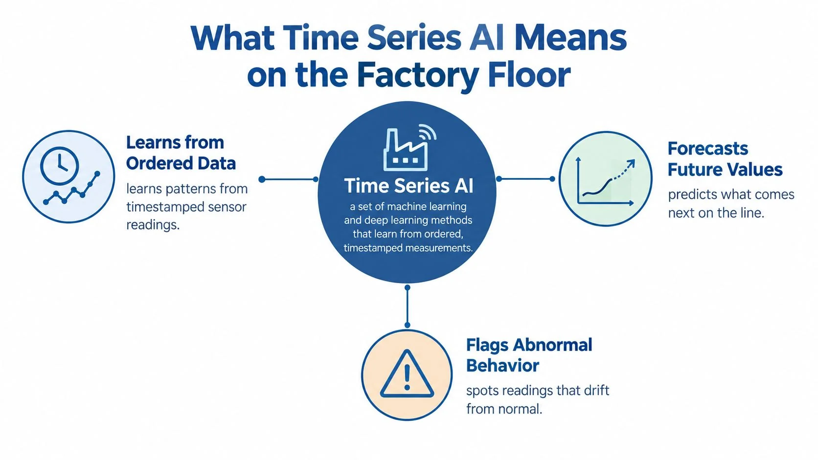
Time series AI is a set of machine-learning and deep-learning methods that learn from ordered, timestamped measurements to forecast future values, flag abnormal behavior, or estimate remaining useful life. The counterintuitive finding for manufacturers is that a larger, more complex model isn't necessarily more accurate. Industrial comparisons below show why plants should choose models by operating regime, forecast horizon, and calibration, not architecture alone.
Table of Contents
- What Time Series AI Means on the Factory Floor
- Method Families Matched to Manufacturing Tasks
- Choosing Models by Horizon and Signal
- Foundation Models and When to Trust Them
- Evaluation Metrics That Predict Plant Outcomes
- Case Study Highlights and What They Prove
- Confirm Scope and Start a Baseline Pilot
What Time Series AI Means on the Factory Floor
Time order carries information. A rising temperature after a load change means something different from the same temperature during steady production. Shuffling observations or validating on randomly mixed neighboring windows can erase that context or make performance look better than it is.
Consider these illustrative factory streams:
- Spindle vibration sampled every second: Useful for tracking changes in machine behavior, provided the acquisition process preserves the frequencies relevant to the fault.
- Furnace temperatures logged every minute: Useful for forecasting thermal drift and identifying deviations from recipe-dependent behavior.
- Hourly Overall Equipment Effectiveness values: Useful for anticipating production losses, although aggregation can conceal brief stops.
Check telemetry before choosing algorithms
Start in the historian, SCADA system, or MES. Inspect timestamp consistency, missing samples, sensor replacements, and idle periods recorded as zeros. Confirm that startup, changeover, and shutdown events have usable tags.
History must cover the seasonal or degradation behavior you're trying to validate, with enough later observations reserved for testing. A partial failure trajectory can't establish whether an RUL estimate remains useful through failure.
Classical forecasting methods such as exponential smoothing and ARIMA remain part of this workflow. AI extends those approaches rather than making them obsolete.
For maintenance teams connecting telemetry to work orders, the E & I Sales maintenance guide offers practical context for predictive-maintenance planning.
Start with the output: Name the forecast, anomaly score, or RUL estimate you need, identify its data source, and specify who will act on it.
Method Families Matched to Manufacturing Tasks
Method families by manufacturing task
| Task | Method families | Typical horizon | Data you need |
|---|---|---|---|
| Demand forecasting | Seasonal-naive, ETS, ARIMA, gradient boosting, hybrids | Days to weeks | As a pilot starting specification, 2+ years of history, calendar and promotion inputs |
| Sensor and OEE forecasting | Linear-exponential models, gradient boosting, LSTM, Transformer | 8 to 72 hours | Hourly data with a seven-day input window as a candidate configuration |
| Remaining useful life (RUL) | Random forest, XGBoost, deep sequence models | Cycles or weeks | Run-to-failure history with maintenance records |
| Anomaly detection | Forecast-residual thresholds, isolation forest, autoencoders | Real time | Labeled events or a clean normal-operation baseline |
| Zero-shot forecasting | Time series foundation models | Any requested horizon, subject to model limits and validation | Little or no target training history; recent context for forecasting |
Treat the table as a candidate-selection guide, not a guarantee of sufficient data. Demand history must represent the relevant calendar patterns; failure history must include the degradation mechanisms you expect to detect. Zero-shot forecasting removes task-specific training, not the need for target-plant testing.
The M4 findings summarized in the decoder-only forecasting model article showed that all pure machine-learning submissions were less accurate than the combination benchmark, while the winning hybrid improved accuracy over that benchmark by 9.4% and over Naïve 2 by 16.2%. That's a strong reason to retain statistical controls and test combinations rather than assume deep learning deserves deployment.
Every forecasting candidate should beat a seasonal-naive or exponential-smoothing baseline on the same validation period before it earns a pilot.
For maintenance-specific selection, compare the output requirements described in predictive maintenance models. A failure classifier, an RUL estimator, and a sensor forecast aren't interchangeable, even when they use the same telemetry.
To connect model outputs with operational workflows, devPulse's discussion of predictive insights for digital transformation provides broader planning context. Keep the plant's acceptance criterion concrete: enough improvement to justify integration, inference, and ongoing maintenance.
Choosing Models by Horizon and Signal
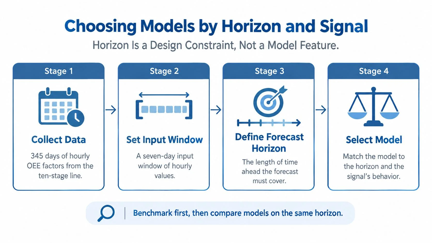
Horizon is a design constraint, not a model feature. A forecast that arrives too late for parts procurement doesn't support maintenance planning, however low its error.
The following evidence connects model choice to specific signals and decision windows.
Horizon and signal decisions with the evidence behind them
| Horizon or signal | Decision it supports | Reported evidence | Validation to use |
|---|---|---|---|
| 8 to 72 hours, OEE factors | Dispatching and intervention scheduling | In the antenna-assembly benchmark, PDFLinearEWA achieved RMSE of 0.169, 0.173, and 0.173 at 8, 24, and 48 hours; another model led at 72 hours | Rolling-origin, error per horizon |
| Up to 10 days, paper press equipment | Labor planning, parts ordering, planned shutdown | The paper-press case study reported good accuracy up to 10 days ahead after preprocessing and outlier treatment | Blocked time splits at the planning horizon |
| Hot-side heat-exchanger pressure, AV5 furnace | Cooling-circuit maintenance | The AV5 cooling-system study found Prophet best for this pressure signal, DES best for hot- and cold-side temperatures, and ARIMA best for cold-side pressure | Blocked cross-validation with MSE, RMSE, MAE |
| Hot- and cold-side temperatures, AV5 furnace | Temperature-limit management | Double exponential smoothing was the selected method | Rolling-window validation |
| Cold-side pressure, AV5 furnace | Pressure-limit management | ARIMA was the selected method | Rolling-window validation |
The antenna-line evaluation used hourly OEE factors and a historical input window. Its practical lesson isn't that PDFLinearEWA should run every plant. It's that model rankings can change as the forecast extends further ahead.
Turn the decision into a test specification
- Name the action and lead time. Include approval, parts, labor, and shutdown coordination.
- Set the forecast horizon from that lead time, not from the model's default configuration.
- Separate signals and assets. Don't let an easy temperature channel hide poor pressure forecasts.
- Choose a baseline and a small candidate set per signal.
- Use rolling-origin or blocked splits. Fit on earlier observations and evaluate later ones.
- Report error separately at each operational horizon.
- Compare deployment effort. Include inference cost, retraining, and feature availability.
- Connect the forecast to an action threshold, such as a predicted process-limit crossing.
The same lead-time discipline applies to AI for demand forecasting, where procurement and production scheduling may require different forecast windows.
Foundation Models and When to Trust Them
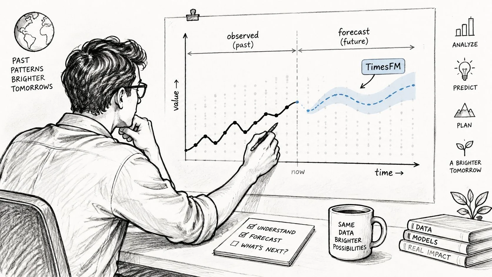
Zero-shot forecasting promises predictions for a series without task-specific training. That's useful when a plant lacks the labeled history needed to fit a specialized model, but it doesn't establish transferability.
TimesFM reportedly outperformed most statistical methods and matched or exceeded target-trained DeepAR and PatchTST in zero-shot evaluations; the NeurIPS GIFT-Eval presentation describes an evaluation benchmark spanning 28 datasets, more than 144,000 series, and 157 million observations. Broad evaluation helps screen candidates, but it doesn't reproduce your product mix, control logic, or maintenance practices.
Test transfer rather than assuming it
Under distribution shift, a domain-specific model with 49.5K parameters outperformed a fine-tuned TimesFM model with more than 500 million parameters, according to the foundation-model comparison summary. Model size isn't a substitute for fit.
Build a transfer test around actual deployment boundaries:
- Across assets: Hold out machines with different wear histories or sensor installations.
- Across plants and products: Reserve a site or product family that wasn't used for tuning.
- Across maintenance regimes: Evaluate behavior before and after overhaul or component replacement.
- Across telemetry conditions: Test gaps, irregular sampling, and zero-heavy idle periods.
Many foundation-model interfaces expect regular observations. Resampling can make telemetry compatible, but interpolation mustn't turn a shutdown or failed sensor into an apparently healthy signal.
Deployment judgment: Use foundation models as fast candidates for data-scarce plants. Retain local models when they perform better on target assets and remain easier to calibrate and maintain.
Evaluation Metrics That Predict Plant Outcomes
Average forecast error can look acceptable while the model fails during the operating transitions that matter most.
Metrics to report beyond average error
| Metric | What it tells you | Blind spot | Report it as |
|---|---|---|---|
| MAE, RMSE, MAPE | Average forecast-error magnitude | Routine periods dominate | Error per horizon and regime |
| Prediction interval coverage | Whether observed values fall inside the stated probability interval | Point metrics don't measure it | Empirical coverage and interval width per regime |
| Early-warning lead time | Time from first qualifying alert to failure | Doesn't capture false alarms | Median and minimum lead time per failure mode |
| False alarms per operating hour | Operator alert burden | Doesn't capture missed failures | False-alert events divided by operating hours, per regime |
| Missed failures | Failures without a qualifying prior alert | Sensitive to alert threshold | Count and percentage per failure mode |
| Error by operating regime | Performance during startup, changeover, shutdown, recipe change | Requires regime labels | Separate results per regime |
Measure error and uncertainty separately
MAE summarizes absolute error. RMSE penalizes larger errors more strongly. MAPE expresses error relative to the actual value, but becomes unsuitable around zero, including idle production signals.
Calibration answers a different question: do prediction intervals contain actual outcomes at their stated frequency? Compare coverage with interval width, because a very wide interval can cover observations without supporting a useful decision.
A traffic-forecasting analysis reported transition-regime MAE of 11 mph versus 3 mph overall, while empirical coverage of nominal 90% intervals fell as low as 55%. That's not manufacturing evidence, but it illustrates why plant teams should test startup, shutdown, tool-wear transitions, and sensor recalibration separately.
Score the alert policy operators will use
Lead time should begin at the first alert that meets the deployed persistence and threshold rules, not at an isolated spike discovered afterward. Count repeated alerts consistently, and distinguish an alert episode from every above-threshold sample.
A missed failure is an event without a qualifying warning inside the actionable maintenance window. Set that window with maintenance planners before testing. Otherwise, teams can make results look favorable by redefining what counts as timely.
For asset generalization, the C-MAPSS evaluation discussion describes simulated engine degradation and distinguishes FD001's single fault mode from FD003's two fault modes. Split by asset, not random rows, so neighboring cycles from the same machine don't leak into both training and test sets.
Label regimes using MES recipe codes, machine-state tags, and shift logs. If those labels are missing, add them before scoring. A model passes only when its deployed alert policy meets maintenance-defined lead-time, false-alarm, and missed-failure limits in the regimes that matter.
Case Study Highlights and What They Prove
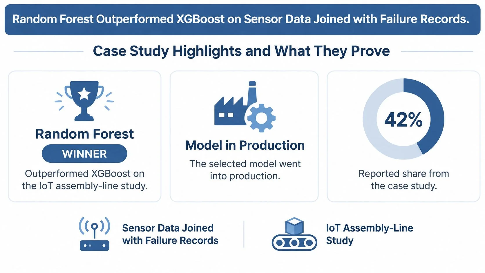
In the IoT assembly-line study, random forest outperformed XGBoost, the selected model entered production, and the system prevented approximately 42% of actual production-line failures. Read that as an outcome from one factory and production context, not a transferable savings assumption.
Reference cases, reported results and caveats
| Case | Asset and signal | Reported result | Caveat |
|---|---|---|---|
| IoT assembly-line study | Line sensors with failure or maintenance records | Production deployment and prevented failures | One factory and production context |
| Pulp-and-paper press study | Press telemetry after outlier treatment | Useful forward prediction of equipment behavior | Planning value requires sufficient parts and labor lead time |
| AV5 furnace cooling study | Hot- and cold-side temperature and pressure | DES, Prophet, and ARIMA won on different signals | A winning algorithm isn't automatically transferable |
| NASA C-MAPSS benchmark | Simulated turbofan trajectories | Test bed for RUL and fault detection | Simulated trajectories aren't operating-plant outcomes |
Audit outcomes before using them in a business case
Check the actionable horizon first. A warning only creates value when the plant can intervene before the failure or quality excursion.
Next, identify the baseline the model beat and whether the validation preserved chronology. Then establish whether the operational result is vendor-reported, independently assessed, or supported only by retrospective predictions.
For a separate implementation reference, Faberwork LLC's time series data success story can inform questions about data infrastructure. Keep architecture evidence separate from evidence of prevented failures or financial return.
Use a case database to filter by industry and use case, then compare horizon, validation method, and outcome definition. Don't copy a reported improvement into your ROI model unless the plant conditions and measurement process are genuinely comparable.
Confirm Scope and Start a Baseline Pilot
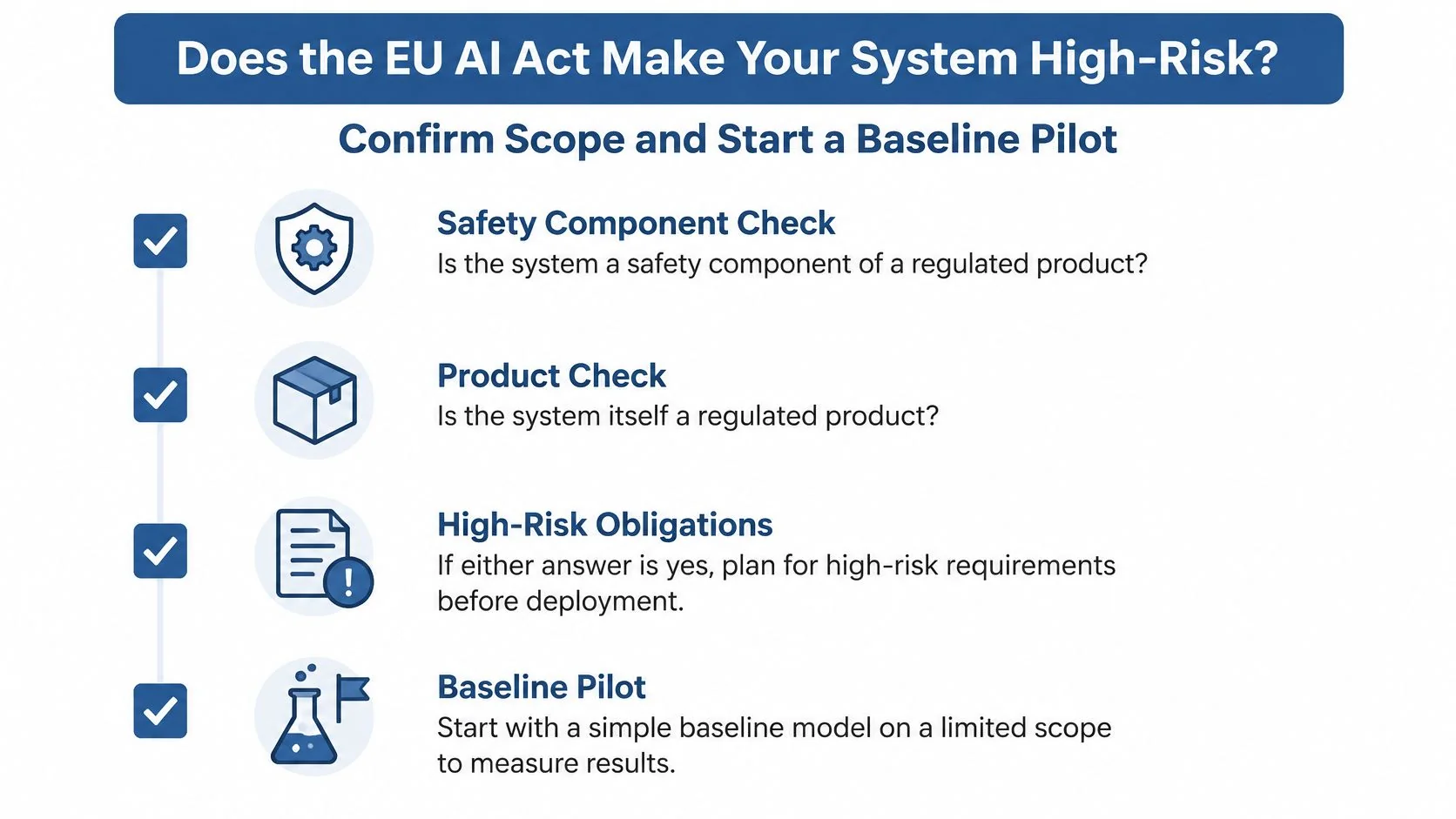
Resolve the safety boundary before deployment. The EU AI Act service guidance describes high-risk conditions when an AI system is a safety component of a regulated product, or is itself such a product, and the product requires third-party conformity assessment.
The guidance includes monitoring abnormal behavior and identifying maintenance or inspection needs for safety-related parts where failure could cause harm. A downtime advisory and a decision about replacing a safety-related component can therefore require different governance. Don't treat the simplified checklist as a substitute for assessing the complete legal conditions.
Run a bounded acceptance pilot
- Define the output and owner. Specify the forecast, anomaly score, or RUL estimate and the decision it triggers.
- Derive the horizon from the action's required lead time.
- Build the baseline first. Test statistical controls and a small candidate set on the target asset using chronological evaluation.
- Record regime-level error, interval calibration, warning lead time, false alerts, and missed failures.
- Document the operating controls. Include intended use, affected machinery, alarm logic, human override, sensor provenance, validation evidence, and maintenance decisions.
- Decide go, revise, or stop against thresholds fixed before testing.
Use a manufacturing data analytics review to assign ownership of telemetry quality and operational reporting. A model without those owners won't remain dependable after sensor changes or process adjustments.
Choose a workflow and baseline now, then compare documented AI for manufacturing use cases before committing model budget. AI for Manufacturing is one option alongside original technical papers and vendor documentation: its searchable case database lets teams compare implementations by industry, use case, technology, and reported outcomes. Bring a shortlist of comparable cases to maintenance, production, and engineering, and agree on the acceptance test for your plant.
