Random Forest in Machine Learning for Manufacturing AI
Master random forest in machine learning with practical guidance on tuning, evaluation, and deployment. Learn how to apply it to manufacturing AI use cases.
Written by AI for Manufacturing

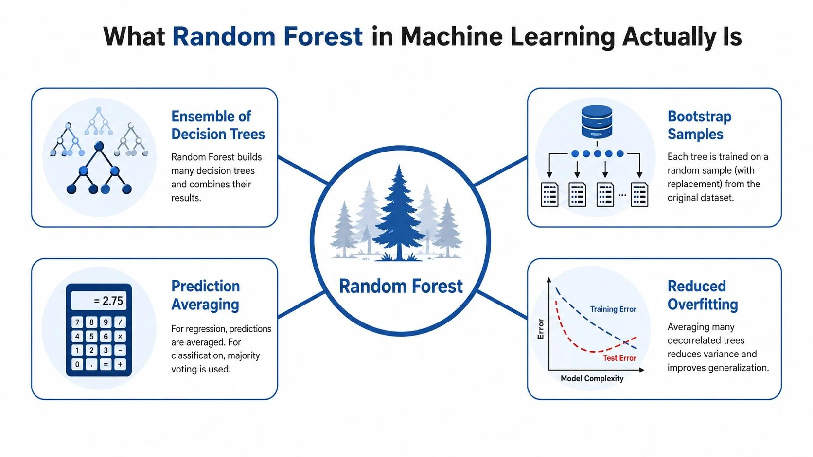
Random forest in machine learning is an ensemble method that trains many decision trees on bootstrap samples of the data, then combines their predictions by majority vote for classification or averaging for regression. It also introduces random feature subsetting at each split, which decorrelates trees and reduces variance and overfitting compared with a single decision tree. In manufacturing work, that matters because noisy sensors, unstable processes, and mixed data types are the norm, not the exception.
The advice I challenge most often is that you should jump straight to a more complex model. In plant settings, random forest is often the better first model because it is resilient, interpretable enough to debug, and forgiving when your data are messy. It also forces a practical conversation about the core problem, whether that is a rare failure, a drifting process, or a quality escape that only shows up under specific operating conditions.
Table of Contents
- What Random Forest in Machine Learning Actually Is
- How Bagging and Feature Randomness Reduce Overfitting
- Key Hyperparameters and Tuning Trade-Offs
- Handling Imbalanced Data for Rare Failure Detection
- Evaluation Metrics That Connect to Shop-Floor Decisions
- Implementation Checklist from Data Prep to Deployment
- Applying Random Forest to Manufacturing AI Use Cases
What Random Forest in Machine Learning Actually Is
Random forest in machine learning is an ensemble of decision trees built on bootstrap samples of the training data, with random subsets of features considered at each split. The trees are grown to their largest extent in the original formulation, then combined by majority vote for classification or by the mean prediction for regression. Because each tree sees a different slice of the data and a different slice of the features, the ensemble is usually more stable than a single tree, which is exactly why it tends to generalize better on messy industrial data. That behavior is documented in the original Breiman formulation of random forests, which emphasizes both bootstrap sampling and random feature selection as the core design choices that reduce variance and overfitting relative to a single tree (Breiman's random forest page).
Why manufacturing teams reach for it first
Factory data usually mixes continuous signals, counts, statuses, operator inputs, and categorical context. Random forest handles that mix without demanding the kind of heavy preprocessing that some other models need. It's a practical fit for predictive maintenance, quality prediction, and process optimization, especially when you want a baseline that works before you spend weeks building a more elaborate stack.
The model also gives you feature importance, which is useful when process engineers ask which sensors matter and why a part was flagged. That matters more than it sounds, because adoption in manufacturing often depends on whether the model can survive scrutiny from the people who run the line.
Practical rule: If the process is noisy, the labels are imperfect, and the first goal is a dependable baseline, random forest usually deserves a serious look before neural networks.
A useful way to think about it is this. Random forest doesn't try to make one perfect tree, it tries to make many imperfect ones that fail in different ways. The ensemble effect is what makes the method durable in production environments where one sensor drifts, one tool wears faster than expected, or one shift logs data differently than another.
How Bagging and Feature Randomness Reduce Overfitting
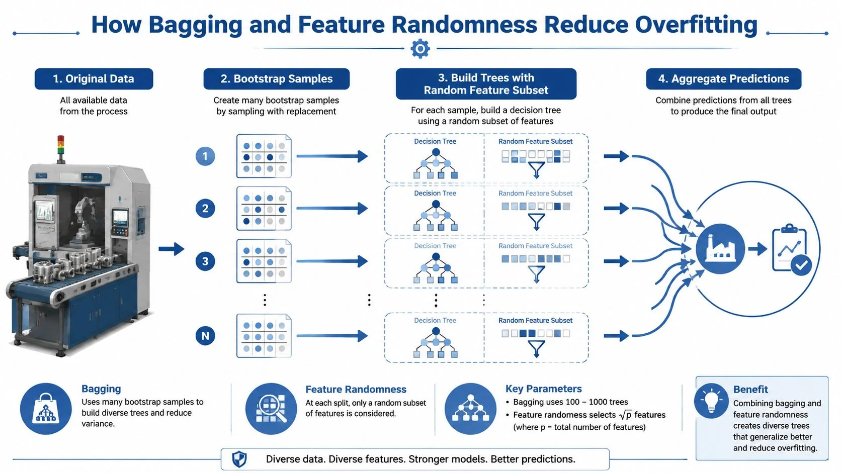
The two mechanisms that matter most are bagging and random feature selection. Bagging, short for bootstrap aggregating, trains each tree on a resampled version of the dataset. Feature randomness then limits how much any one dominant sensor can steer the split decisions, which keeps the trees from becoming clones of each other. That diversity is the whole point.
A tool-wear example from the shop floor
Suppose you're predicting tool wear from vibration, temperature, and spindle load. A single decision tree can latch onto one noisy vibration spike and treat it as a meaningful rule. That looks clever in training, then falls apart when a different machine, tool holder, or coolant setting changes the signal pattern.
Random forest softens that problem because no tree gets to see the exact same bootstrap sample, and no split gets to consider every feature. The result is that local quirks matter less. In manufacturing terms, the model is less likely to confuse a temporary process wobble with a real wear signature.
Why decorrelation matters more than perfection
Many teams focus too much on making one tree “smart.” That's the wrong objective. What you want is a group of trees whose errors aren't highly correlated, because then the ensemble can average away instability. That's the reason random forest often performs well on noisy sensor streams where individual trees would overreact.
An internal validation signal helps here too. Many implementations expose out-of-bag error, which uses the data points that were not included in a tree's bootstrap sample as a built-in check. You don't need a separate validation set just to get a first read on performance, although you still need a proper holdout when the process is time-dependent.
The educational technical note in the brief describes random forests as commonly trained with hundreds of trees, often 500 to 1000, while selecting only a subset of features at each node (technical note on random forest practice). In production, the reason this matters is simple. More trees usually lower variance, but the gains shrink once out-of-bag error stops moving, and the compute cost keeps rising.
Key Hyperparameters and Tuning Trade-Offs
The hyperparameters that matter most in production are the number of trees, max features per split, max depth, and minimum samples per leaf. The main trade-off is straightforward. More trees usually make the model more stable, but they also raise compute and memory linearly, which is a real constraint when the model has to run near the line or inside a latency budget.
What to tune first
Start with the tree count and the feature subset size. If the forest is too small, prediction variance stays high. If the feature subset is too large, trees become too similar and you lose the decorrelation benefit. Max depth and leaf size then control how finely each tree can fit the data, which matters when you have sparse failures or highly segmented operating regimes.
A good production habit is to watch out-of-bag error as trees are added. Once that curve stabilizes, more trees are usually giving you diminishing returns, not meaningful business value. That's the point where engineers should stop tuning for elegance and start asking whether the current model meets latency and memory limits.
| Random Forest Hyperparameter Effects at a Glance | |||
|---|---|---|---|
| Hyperparameter | Effect on Accuracy | Effect on Training Time | Effect on Inference Latency |
| Number of trees | Usually improves stability, then levels off | Increases roughly linearly | Increases roughly linearly |
| Max features per split | Too high can reduce tree diversity, too low can underfit | Moderate effect | Moderate effect |
| Max depth | Deeper trees can fit more detail, but may overfit | Increases with complexity | Can increase noticeably |
| Minimum samples per leaf | Larger leaves smooth noise, smaller leaves fit more detail | Usually modest effect | Usually modest effect |
What usually stays near default
Many teams leave the split criterion and other lower-level controls alone unless the data are unusual. That's fine. The bigger wins come from getting the forest size and split constraints right for your plant. If your model is deployed on an edge device or inside a tightly scheduled SCADA-linked workflow, latency often matters more than squeezing out a marginal score improvement.
If the gain from another tuning pass is hard to explain to a supervisor in terms of fewer false alarms or faster decisions, it probably isn't worth the extra complexity.
In manufacturing, tuning is not about chasing the prettiest model. It's about finding the smallest model that stays useful under real cycle times, real data volumes, and real maintenance constraints.
Handling Imbalanced Data for Rare Failure Detection
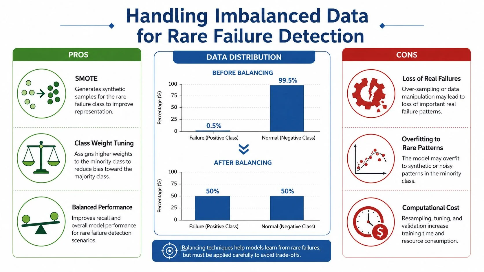
Random forest can look strong on paper and still fail badly on rare events. That's the trap with imbalanced manufacturing datasets. If 99 out of 100 records are normal operation, a model can get away with predicting normal almost all the time and still appear accurate. That's useless when the actual job is finding the one scrap condition, quality escape, or impending failure that matters.
Why default majority vote breaks down
The default majority-vote story is fine for balanced problems, but it doesn't solve low-prevalence events. The Berkeley technical report in the brief explicitly addresses imbalance by changing the bootstrap procedure so the minority and majority classes are sampled equally, which is a strong signal that standard random-forest training can be weak when the target event is rare (Berkeley technical report on random forests for imbalance). That's the manufacturing reality behind the theory.
For scrap prediction, equipment-failure prediction, and quality escapes, the positive class is often tiny. In those settings, balanced bootstrap sampling is one of the most practical fixes because it forces each tree to see enough rare examples to learn something meaningful. Class weighting can also help when you want to preserve the original class structure but push the model to care more about failures. Threshold adjustment comes later, after training, when you want to trade false alarms against missed events.
What works and what doesn't
Balanced sampling is useful when the minority class is underrepresented enough that the trees barely see it. Class weights are useful when you want a lighter-touch adjustment. Threshold tuning is useful when the model ranks cases well but the default cutoff is too conservative for operations.
- Balanced bootstrap sampling: Use it when rare failures are the main target and the trees need more exposure to positive examples.
- Class weighting: Use it when you want to keep the dataset intact but shift the model's attention toward failures.
- Threshold tuning: Use it when the ranking is acceptable, but the default decision cutoff misses too many events.
What doesn't work is pretending accuracy means safety. A model that predicts “normal” all day may still be the wrong model.
Operational rule: For rare failures, judge the model by whether it surfaces the events your maintenance or quality team would actually act on, not by whether it looks tidy in a scorecard.
Evaluation Metrics That Connect to Shop-Floor Decisions
Accuracy is the wrong headline metric for most manufacturing problems. It hides the cost of missed failures and over-alerting. On the shop floor, the key question is not whether the model gets the majority class right, it's whether it helps operators and engineers make better calls under time pressure.
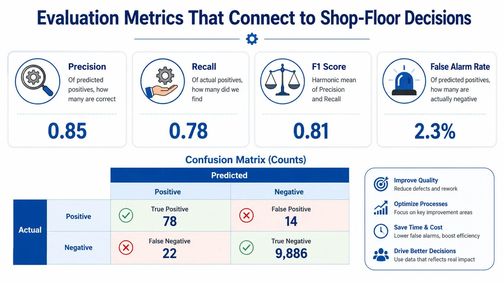
The metric cards in the graphic reflect the kind of scorecard that's useful. Precision tells you how many flagged parts are bad. Recall tells you how many bad parts you caught. F1 score balances those two. False alarm rate matters because too many nuisance alerts burn trust fast. The confusion matrix then makes the trade-offs concrete, which is why I always prefer it over a single headline number.
Match the metric to the decision
For quality inspection, precision matters when each flagged part requires expensive manual review. Recall matters when missing a defect is far more costly than checking an extra part. In maintenance, recall often carries more weight because the missed failure is the one that shuts a line down or damages equipment.
A model can also rank cases reasonably well while needing a threshold change before it becomes operationally useful. That's why ROC-AUC is helpful for comparing models across possible cutoffs, but it still doesn't replace the confusion matrix. The scores matter less than how they translate into action.
The internal guide on manufacturing quality metrics offers a useful companion framework for turning these numbers into operational language, and it's worth using alongside any model review process: manufacturing quality metrics guide.
Translate scores into plant decisions
Plant managers don't need a lecture on probability. They need to know whether the model catches enough bad cases, creates too many false stops, or can support a staffing decision on the next shift. That means presenting precision, recall, and false alarm rate together, then discussing what each one means for inspection load, downtime, and risk.
For manufacturing AI, the metric is only valuable if it changes a decision. If it doesn't help someone stop a defect, schedule service, or prioritize an intervention, it's just a number on a dashboard.
Implementation Checklist from Data Prep to Deployment
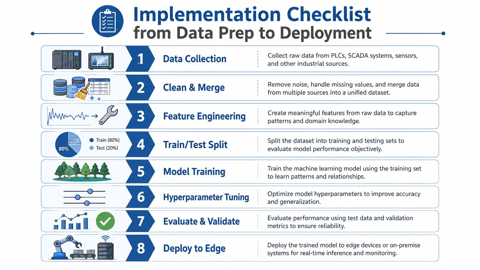
A good random forest project in manufacturing starts long before training. The hardest failures I've seen usually come from weak data preparation, not from the algorithm itself. PLCs, SCADA systems, historian exports, and manual logs rarely line up cleanly, and time ordering matters more than teams expect.
Build the data foundation first
Start by collecting data from the control stack, then clean and merge records so timestamps, asset IDs, and production context line up. Feature engineering should convert raw time-series signals into meaningful windows, summaries, and lagged variables. That's where a lot of the signal lives, especially when the equipment runs in bursts instead of steady-state cycles.
Time-respecting train-test splitting is essential. Random shuffling can leak future conditions into the past and make the model look better than it really is. If the line changed tooling, suppliers, or recipes over time, the split needs to preserve that history.
The manufacturing data collection guide is a useful companion when you're pulling those sources together: manufacturing data collection guide.
Train, validate, then watch drift
After the split, train the forest, tune the key hyperparameters, and validate with both out-of-bag error and a holdout set. Then move to deployment with monitoring. That last step is where many projects fail.
- Data Collection: Pull PLC, SCADA, and historian signals into one governed dataset.
- Clean and Merge: Align timestamps, remove duplicate records, and resolve bad tags.
- Feature Engineering: Turn raw sensor streams into lagged, rolling, and event-based features.
- Train and Test Split: Keep temporal order intact so future conditions don't leak backward.
- Model Training: Build the forest with a sensible starting tree count and feature subset.
- Hyperparameter Tuning: Adjust tree count, depth, and leaf size only where the data support it.
- Evaluate and Validate: Compare out-of-bag error, holdout metrics, and confusion matrices.
- Deploy to Edge: Monitor performance where the model is used.
Deployment monitoring should focus on drift, not just uptime. If sensor distributions change, process settings shift, or the supplier mix changes, the model may stop being trustworthy even if the software still runs. In plants I've worked with, that's the moment to retrain or at least revalidate before the model becomes a liability.
Applying Random Forest to Manufacturing AI Use Cases
Random forest fits best where the data are noisy, the labels are uneven, and the business needs a dependable baseline quickly. That includes predictive maintenance for rotating equipment, quality prediction in casting or molding, process parameter optimization for CNC machining, and energy consumption forecasting when the input mix changes over time. The main requirement is disciplined feature engineering and a careful validation plan.
For teams evaluating where to start, the best comparison point is documented plant evidence, not vendor promises. The AI for Manufacturing database is built for that kind of benchmarking, with searchable implementations, source-linked records, and standardized case summaries that help teams compare use cases before they commit resources. If you're deciding whether random forest belongs in your manufacturing AI roadmap, review the documented cases in the predictive maintenance models collection, then match your data quality, failure rarity, and deployment constraints to what's already been proven in similar industrial settings.
If you're planning a manufacturing AI project, start by checking whether your problem is a noisy baseline problem, a rare-event problem, or a drift problem. Then compare your use case against documented implementations in AI for Manufacturing, so you can choose random forest with evidence instead of guesswork.
