How to Calculate OEE: Formulas, Examples, and AI-Driven Tips
Learn how to calculate OEE with clear formulas, worked examples, and AI-driven tips for plant managers pursuing AI in manufacturing.
Written by AI for Manufacturing

OEE can change without a machine producing a single additional part. If a plant starts capturing previously unlogged minor stops, reclassifies changeovers, or replaces estimated counts with sensor data, the reported score can move because the measurement became more complete. Overall Equipment Effectiveness, or OEE, measures the proportion of planned production time that produces good parts at the ideal rate, using Availability × Performance × Quality. The formula is simple. The data policy behind it is where most programs succeed or fail.
Table of Contents
- What OEE Actually Measures in a Plant
- The Three Components of the OEE Formula
- Worked Examples for Single Shifts and Product Runs
- Aggregating OEE Across Shifts, Lines, and Plants
- Data Sources and Measurement Best Practices
- Common Calculation Pitfalls and How to Fix Them
- Where AI Changes OEE and What to Do Next
What OEE Actually Measures in a Plant
OEE is a ratio of what an asset produced against what it could have produced during a defined production window under ideal conditions, with no stops, no speed loss, and no defects. It doesn't measure how busy a machine looks. That makes it useful because it exposes downtime, hidden speed loss, and quality loss in one KPI.
The standard structure is:
OEE = Availability × Performance × Quality
A commonly cited benchmark places 85% OEE in the world-class range, while reported manufacturing averages sit around 60%, and some benchmark reporting places the top quartile near 75%. These reference points are directional, not universal rules. Product mix, changeover frequency, validated cycle rates, regulatory holds, and the physical process can all limit what a particular asset can achieve. The OEE benchmark discussion from Fabrico also reinforces why a target only makes sense when the underlying calculation method is consistent.
Utilization, throughput, and first-pass yield answer narrower questions:
- Utilization asks how much calendar or available time an asset was in use, but it may not reveal whether the machine ran slowly or produced defects.
- Throughput measures output volume, but it doesn't explain whether lost capacity came from downtime, speed, or quality.
- First-pass yield focuses on accepted output, but it doesn't show how much scheduled time was lost before production reached that output.
Practical rule: Define the asset, product, and production window before collecting numbers. A score without a boundary isn't comparable to anything.
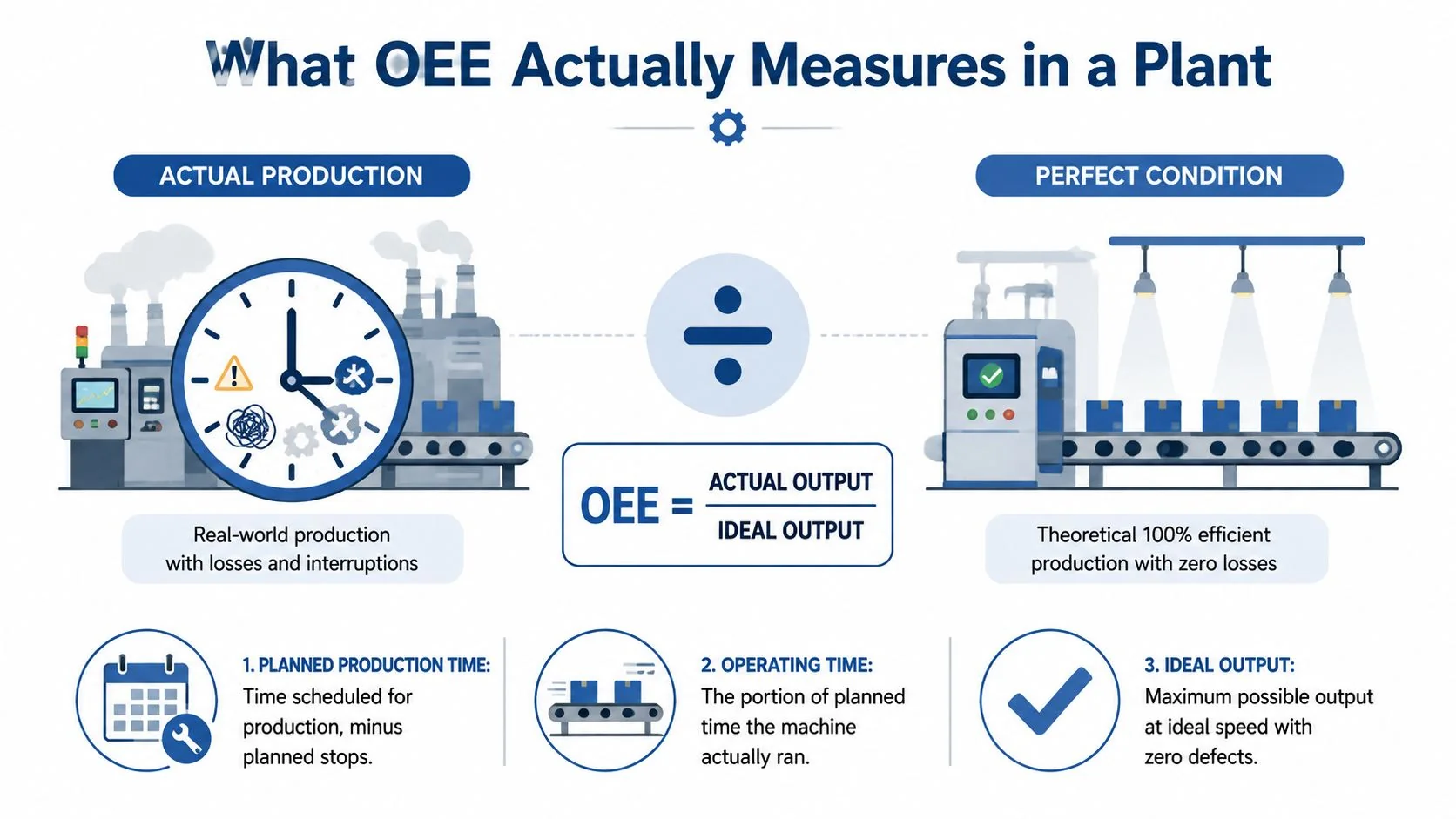
OEE should normally describe a named machine, work cell, or line during a defined run or shift. It isn't automatically a factory-wide metric. That scope decision matters for AI because a model trained on machine-level events can't reliably diagnose a plant-level score if the plant rollup mixes products, shifts, and operating policies.
The Three Components of the OEE Formula
Calculate each component separately, audit its numerator and denominator, then multiply the resulting decimals. Don't average the three percentages, and don't substitute convenient measures for the defined inputs.
Availability
Availability = (Planned Production Time − Downtime) ÷ Planned Production Time
Planned Production Time is the time scheduled for production after scheduled breaks and planned stops are removed. Run Time is what remains after production-time stops are deducted.
Downtime covers events that stop planned production for an appreciable period, usually several minutes, long enough for an operator to record a reason. The OEE factors definition is useful when setting a minimum-duration rule for event detection. Under the original SEMI E10 approach, changeovers are also treated as availability loss when they occur inside the production window. Your plant can adopt a different policy, but it must document and apply that policy consistently.
Performance
Performance = (Ideal Cycle Time × Total Pieces Produced) ÷ Run Time
This component captures reduced speed, idling, and minor stops. The common calculation mistake is using actual average cycle time instead of Ideal Cycle Time. That error makes a slow operating condition look normal and can inflate Performance.
Ideal Cycle Time should come from a governed engineering or process standard, not a live average. It must be specific to the SKU or product family when products run at different rated speeds. If the baseline is allowed to drift downward, future improvement becomes harder to see.
Quality
Quality = Good Pieces ÷ Total Pieces Produced
Good Pieces are units that pass the defined quality gate without being counted as scrap or accepted rework. Reworked parts may eventually ship, but they weren't right first time. Keep that distinction visible if OEE is being used to expose process effectiveness.
| Component | Formula | Loss Category Captured | Interpretation Rule |
|---|---|---|---|
| Availability | (Planned Production Time − Downtime) ÷ Planned Production Time | Breakdowns, stops, setup, and adjustments | Shows how much scheduled time was actually available for production |
| Performance | (Ideal Cycle Time × Total Pieces) ÷ Run Time | Idling, minor stops, and reduced speed | Compares actual output against the ideal rate while running |
| Quality | Good Pieces ÷ Total Pieces Produced | Process defects and startup or reduced-yield losses | Measures first-pass good output |
| OEE | Availability × Performance × Quality | Combined effect of all three loss groups | Multiply decimal values, then convert the result to a percentage |
The six big losses framework maps breakdowns and setup losses to Availability, idling and reduced speed to Performance, and process defects plus startup losses to Quality. That mapping should also appear in your AI event taxonomy.
Worked Examples for Single Shifts and Product Runs
The fastest way to learn how to calculate OEE is to use the same sequence every time: define planned time, subtract downtime, calculate each factor, multiply the decimals, and then identify the dominant loss.
Scenario one, one product on one shift
Assume an 8-hour shift, with no additional planned stops specified. Planned Production Time is therefore 480 minutes. The asset loses 47 minutes to unplanned downtime, produces 980 pieces, and records 12 rejects. The operating rate is 10% slower than the ideal rate, so Performance is 90.0%.
- Availability: (480 − 47) ÷ 480 = 90.2%
- Performance: 90.0%
- Quality: (980 − 12) ÷ 980 = 98.8%
- OEE: 0.902 × 0.900 × 0.988 = 80.1%
The largest visible loss is Availability. Breakdowns and other stops should be separated before corrective action, because the first response differs for equipment failure, material waiting, and operator intervention.
Scenario two, two SKUs and a changeover
A single asset runs two SKUs during the same shift. The first SKU has an ideal cycle time of 30 seconds and produces 600 pieces. The second has an ideal cycle time of 45 seconds and produces 400 pieces. The correct ideal-time numerator is:
(30 × 600) + (45 × 400) = 36,000 seconds
That is equivalent to a piece-weighted ideal cycle time of 36 seconds, not a simple average of the two cycle times. If the shift includes a 35-minute changeover, classify it according to the plant's documented policy. Under the SEMI E10-style treatment described earlier, it reduces Availability when it occurs during planned production.
This example matters because averaging SKU cycle times can overstate or understate Performance. A product with more pieces should contribute more to the ideal-time numerator. Keep the full run-level data, then aggregate the numerators and denominators.
Scenario three, a high OEE with a hidden speed problem
Suppose a line reports 82% OEE, but Performance is seven percentage points below what the line could achieve because short jams and repeated resets are recorded as “running.” The score may look strong while the line loses recoverable capacity through minor stops.
The first corrective action is event capture, not a broad maintenance campaign. Separate micro-stops from true running time, classify the stop reasons, and determine whether the repeated events come from sensors, feeding, controls, or operator adjustments.
| Scenario | Planned Time (min) | Downtime (min) | Pieces Produced | Reject Count | Ideal Cycle Time (sec) | Availability % | Performance % | Quality % | OEE % |
|---|---|---|---|---|---|---|---|---|---|
| One product, one shift | 480 | 47 | 980 | 12 | Governed standard | 90.2 | 90.0 | 98.8 | 80.1 |
| Two SKUs with changeover | Defined by shift policy | 35 changeover plus other stops | 1,000 combined | Must be recorded by SKU | 30 and 45 | Calculate from run data | Use weighted ideal-time numerator | Good ÷ total | A × P × Q |
| High OEE with minor stops | Defined production window | Recorded stops only | Line total | Line total | Governed standard | Reported from captured stops | 7-point drag identified | Calculate from first-pass output | 82.0 reported |
The Six Big Losses diagnosis changes with the evidence. Scenario one points first to breakdowns or other Availability losses. Scenario two points to setup and adjustment governance. Scenario three points to idling, minor stops, and reduced speed.
Aggregating OEE Across Shifts, Lines, and Plants
Aggregation is where many OEE programs break down. A simple average of shift percentages treats a short run and a long run as equally important, even when their planned times, output volumes, products, and loss patterns differ.
Use the underlying numerators and denominators instead.
The correct rollup
For a group of product runs, calculate:
- Availability = ∑ Run Time ÷ ∑ Planned Production Time
- Performance = ∑(Ideal Cycle Time × Total Parts) ÷ ∑ Run Time
- Quality = ∑ Good Parts ÷ ∑ Total Parts
- Rolled-up OEE = Availability × Performance × Quality
This method preserves run length and product-specific ideal rates. It's the aggregation approach recommended by OEE.com's calculation guidance, which specifically cautions against treating OEE as a simple arithmetic average across lines or shifts.
A three-shift report can show why this matters. Imagine Shift 1 reports 70%, Shift 2 reports 78%, and Shift 3 reports 86%. A naive average gives 78.0%, but a weighted calculation may differ by 4 to 8 points depending on the planned time, run time, counts, ideal cycle times, and reject totals behind each shift. The exact plant result comes from the raw data, not from the displayed shift percentages.
| Method | Shift 1 | Shift 2 | Shift 3 | Reported Plant OEE |
|---|---|---|---|---|
| Simple average of displayed OEE | 70% | 78% | 86% | 78.0% |
| Weighted component rollup | Underlying run data | Underlying run data | Underlying run data | A × P × Q from summed inputs |
A good shift can hide a bad one if managers look only at the average. That's especially dangerous when a low-volume shift runs an easy SKU while a high-volume shift handles difficult products and frequent changeovers.
Product and policy controls
For mixed-SKU production, either track OEE separately by part number or normalize each run against its governed SKU rate before rolling up. Don't compare a product with a slower design rate against a product with a faster rate using one unqualified cycle-time standard.
Changeover treatment must also match across shifts and sites. If one supervisor removes changeovers from Planned Production Time while another counts them as Availability loss, the comparison is invalid even if both teams use the same formula.
Data Sources and Measurement Best Practices
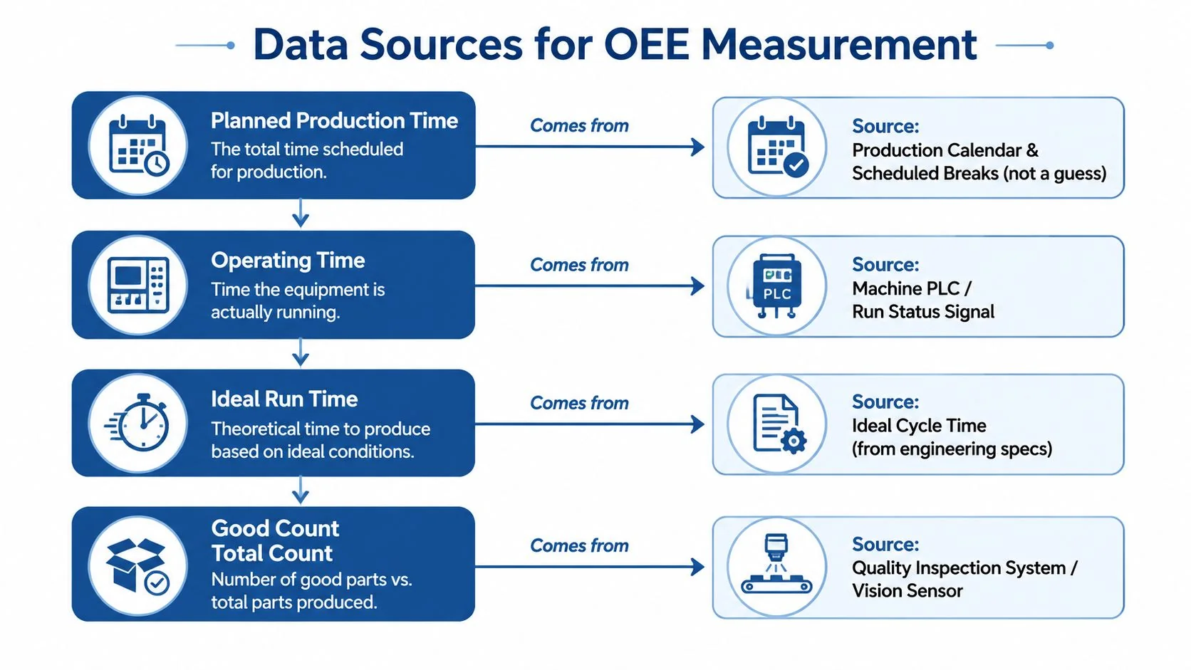
The formula can be mathematically correct and operationally misleading if the inputs are guessed. Planned Production Time should come from the production calendar and scheduled breaks. Operating Time should come from PLC run or stop signals, machine logs, or an equivalent state source. Counts belong in MES counters, production counters, or vision systems, while Good Units should come from the quality inspection process.
Use a source map that someone can audit:
- Planned Production Time: production calendar, scheduled breaks, and approved planned stops.
- Operating Time: PLC state signals or machine event logs.
- Downtime reasons: operator logs, Andon calls, and CMMS work orders.
- Total and actual output: MES, machine counters, or vision systems.
- Good Units: final inspection, in-process inspection, or a governed sampling method.
A stop threshold is essential. Many plants use a threshold in the 30 to 60 second range, but the right choice depends on the process and the event-capture capability. Whatever threshold you choose, document it, apply it to every shift, and classify below-threshold events as Performance losses when they reduce output.
Manual clipboard reporting often produces 10% to 20% variance against sensor measurement of the same shift, as reported in the Hallam guidance on calculating OEE correctly. That variance can exceed the improvement a team is trying to measure. A practical data foundation should include a single minor-stop taxonomy, SKU-specific ideal cycle times, and a locked data dictionary. Teams evaluating collection architecture can also review manufacturing data collection methods before selecting sensors, PLC integrations, or MES interfaces.
Common Calculation Pitfalls and How to Fix Them
Most bad OEE reports fail because the plant has allowed definitions to drift, not because someone can't multiply three decimals. The following checklist catches the issues that most often distort Availability, Performance, and Quality.
-
Planned maintenance counted as unplanned downtime. If an approved planned maintenance period is inside the production calendar, decide whether it belongs in Planned Production Time. If it shouldn't penalize Availability, carve the Planned Maintenance Period into the planned-stop policy and apply that rule consistently.
-
A theoretical cycle time copied from the OEM nameplate. A nameplate value may not represent a validated operating standard for the product and process. Establish a governed rate using competent operation at rated speed across consecutive good cycles, then document the approved value by SKU.
-
Rework counted as good output. Route reworked units through the same quality gate and keep them out of Good Pieces until they pass the defined first-pass criterion. Otherwise, Quality improves on paper while the process loss remains hidden.
-
Speed loss diluted by batch averaging. Capture cycle time at unit or event level where possible. A fast end of the batch shouldn't cancel out a slow middle of the run.
-
Minutes and hours mixed in Performance. Convert every time input to one unit before calculating. A spreadsheet that combines an ideal cycle time in seconds with Run Time in hours can produce a plausible-looking but invalid result.
Audit habit: Review the time definitions, reason codes, ideal cycle-time approvals, rework treatment, and unit conversions before each management review. A one-page monthly check catches drift earlier than a quarterly argument over the score.
The manufacturing intelligence case study on OEE data accuracy is a relevant example of the type of implementation evidence teams should examine when comparing measurement approaches. The aim is to make every adjustment traceable, not to replace engineering judgment with a dashboard.
Where AI Changes OEE and What to Do Next
AI changes OEE measurement in three practical ways. Automatic state detection can replace incomplete operator stop logs. Vision inspection can surface micro-defects that previously disappeared into broad Quality categories. Predictive models can identify patterns associated with Availability risk before a failure stops production.
The architecture should progress in layers:
- Instrument one high-loss line with available machine-state, current, vibration, or process sensors.
- Record every state change in an MES or event platform, including short stops and manual reason codes.
- Calculate OEE from raw events, preserving the Availability, Performance, and Quality components.
- Compare AI-derived results with manual reporting for a controlled validation period.
- Investigate every gap before scaling, because a higher or lower score may reflect better capture rather than a physical performance change.
A pilot should begin with a governed baseline and one clearly defined product or cell. The formula must still equal Availability × Performance × Quality after automation. AI can improve detection, classification, and prioritization, but it can't repair a loose definition of Planned Production Time or an unapproved cycle-time standard.
Teams assessing predictive maintenance approaches can use predictive maintenance models for manufacturing, while AI for Manufacturing provides a searchable database of documented manufacturing AI implementations with filters for industry, use case, technology, and company size. Use those resources to compare deployment patterns, not to skip local validation.
AI improves OEE accuracy first. The operational value appears when engineers use cleaner event data to find root causes faster, reduce recurring minor stops, prevent avoidable downtime, and protect first-pass quality. That value depends on the aggregation and data governance rules covered above.
Start with one line, one product family, and one agreed data dictionary. Document Planned Production Time, stop thresholds, ideal cycle times, changeover treatment, and rework rules before installing models. Then compare the automated calculation with the current report, investigate every discrepancy, and use the loss breakdown to select the first improvement project.
