Demand Forecasting Accuracy: A Manufacturing AI Guide
Improve demand forecasting accuracy in manufacturing with proven metrics, AI methods, and practical strategies. Learn how to measure, monitor, and optimize
Written by AI for Manufacturing

A foundational benchmark reported average forecast error of 48% plus or minus 1% across the preceding five years, meaning the typical forecast missed nearly half of realized demand despite sustained process improvement efforts (industry forecasting benchmark). Demand forecasting accuracy is the measured closeness between predicted demand and actual demand over a defined horizon, product scope, location, and time bucket. In manufacturing, that measurement matters because a forecast feeds purchasing, production scheduling, capacity planning, inventory positioning, and customer service.
A useful forecast isn't the one with the lowest statistical error. It must be evaluated where a planner makes a decision, interpreted with the right metric, and connected to execution systems that can act on the signal. That's why manufacturing AI teams should treat accuracy as a system design problem, not a contest between algorithms.
Table of Contents
- What Demand Forecasting Accuracy Means
- Industry-Standard Metrics and How to Interpret Them
- Why Better Models Do Not Always Mean Better Outcomes
- Root Causes of Forecast Inaccuracy in Manufacturing
- Practical Strategies to Improve Forecast Accuracy
- Measuring and Monitoring Accuracy Over Time
- Connecting Forecast Accuracy to Manufacturing AI Success
What Demand Forecasting Accuracy Means
Forecast accuracy measures how closely a predicted quantity matches demand that materializes. Teams express the gap through metrics such as MAPE, WAPE, MAD, RMSE, and bias. The result is useful only when the forecast horizon, product scope, location, and time bucket match the decision under review. A weekly SKU-location forecast, for example, should be judged against the production replenishment decision it supports.
The 48% average error benchmark cited earlier shows how persistent forecasting problems remain when product mix, promotions, long planning horizons, and volatile demand interact. An industry benchmark from the Institute for Supply Management also reports substantial variation by category, including about 25% median demand forecast error for food and beverages and around 50% for durable consumer products. These figures are context, not universal targets. Manufacturing AI programs need expectations that reflect the item, plant, and decision being measured.
Point forecasts and probability distributions
A point forecast gives one expected value, such as projected weekly demand for a component. Procurement teams use it to calculate purchase orders, while finite-capacity schedulers use it to propose production quantities. Its simplicity supports execution, but it does not show how widely actual demand may vary.
A probabilistic forecast represents a distribution of possible outcomes. Capacity planners, network designers, and inventory policy owners may need that range because their decisions depend on both expected demand and the risk that demand exceeds available supply. AI helps when it can estimate that uncertainty reliably and connect it to a specific planning action. It creates new problems when planners receive complex probability outputs without clear thresholds, ownership, or system integration.
Accuracy also changes with product lifecycle, demand volatility, forecast horizon, and aggregation. Stable, high-volume products often reach roughly 75% to 85% accuracy, while slow-moving items more commonly sit around 50% to 70%. Manufacturing guidance frequently places MAPE in the 20% to 40% range (RELEX forecast accuracy guidance). Treat these as contextual benchmarks rather than promises.
| Dimension | Definition | Manufacturing Impact |
|---|---|---|
| Horizon | Time between forecast creation and the demand period | Determines whether the signal can affect purchasing, production, or capacity |
| Granularity | SKU, location, product family, plant, or enterprise level | Shows whether the forecast supports the execution decision |
| Forecast type | Point estimate or probability distribution | Separates quantity planning from risk and capacity planning |
| Demand pattern | Stable, seasonal, trending, intermittent, or lumpy | Guides model choice and error thresholds |
| Lifecycle stage | New, mature, declining, or discontinued product | Changes the amount and reliability of historical evidence |
Score forecasts at the SKU-location-time bucket level when that is where MRP, replenishment, or scheduling decisions occur. Corporate revenue aggregates can appear accurate because over- and under-forecasted items cancel out. A manufacturing AI deployment that reports only an enterprise average can therefore conceal the errors causing shortages and excess stock. The demand forecasting use case is most useful when its results are tied to the operational decisions the model is intended to improve.
Industry-Standard Metrics and How to Interpret Them
No single metric answers every planning question. A plant may need a percentage error for portfolio comparisons, an absolute unit error for a critical component, a bias indicator for inventory direction, and service metrics for customer outcomes.
Start with the mechanics
MAPE, or Mean Absolute Percentage Error, averages the absolute percentage error across periods:
MAPE = (1/n) × Σ |(Actual - Forecast) / Actual| × 100%
MAPE is intuitive, but it becomes unstable when actual demand is very small and cannot be calculated cleanly when actual demand is zero. Use it for stable items and comparable segments, but don't let it govern intermittent spare parts or lumpy demand without additional measures.
RMSE, or Root Mean Squared Error, is:
RMSE = √[(1/n) × Σ(Actual - Forecast)²]
Because the errors are squared, RMSE gives greater weight to large misses. That makes it useful when an unusually large deviation on a high-volume line can disrupt production, labor, or supplier commitments.
Bias measures directional error. A simple mean forecast error is:
Bias = (1/n) × Σ(Forecast - Actual)
A positive result indicates over-forecasting under this convention, while a negative result indicates under-forecasting. Bias deserves separate attention because absolute-error metrics can show a moderate result even when a process consistently pushes inventory in one direction.
WAPE, or Weighted Absolute Percentage Error, is defined as:
WAPE = Σ|Actual - Forecast| / ΣActual × 100%
The forecast accuracy metric reference explains why WAPE is more stable than MAPE for portfolio-level analysis. Its weighting means larger-volume items influence the score more strongly. The MAPE and WAPE definitions clarify the practical difference: MAPE gives each observation equal percentage weight, while WAPE weights the portfolio through total actual demand.
Practical rule: Pair WAPE with bias. Positive and negative errors can cancel in an aggregate score, while bias exposes whether the planning process is systematically building too much or too little stock.
Interpret the metric at the decision level
A 30% MAPE on a stable, high-runner SKU may indicate a broken data or planning process. The same score on a new launch may be acceptable because historical evidence is limited and the demand pattern is still forming. Similarly, a product-family-month score can appear strong while SKU-week execution remains poor. Aggregation smooths noise and allows offsetting errors to disappear from view.
Service outcomes complete the picture. Track fill rate, stockout frequency, backorders, schedule changes, inventory days, and expedite activity alongside forecast error. A model that reduces MAPE but increases order volatility isn't necessarily helping the plant.
Why Better Models Do Not Always Mean Better Outcomes
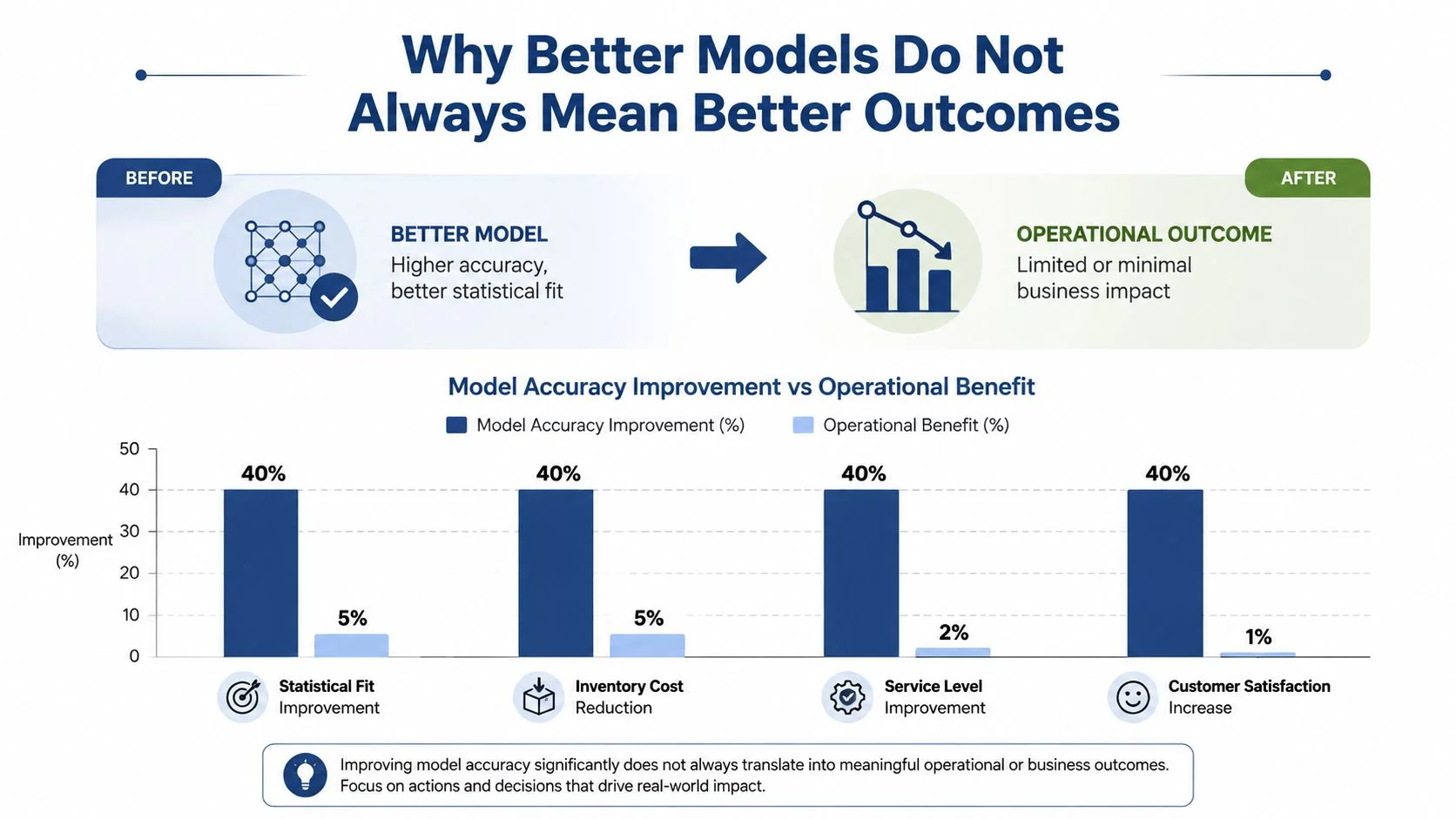
A model can fit historical demand more closely and still make the supply chain less stable. The failure usually occurs after the forecast leaves the data science environment. Procurement batches orders, planners adjust schedules, suppliers operate with lead times, and MRP converts demand into discrete recommendations. Each rule can amplify a small change in the forecast.
A retail supply-chain study found that explanatory variables made forecasts more responsive to changing demand patterns, but also increased the bullwhip effect because replenishment orders became more volatile (study on explanatory variables and bullwhip effects). The manufacturing implication is direct: validate not only MAPE or MAD, but also order variability, bias, inventory oscillation, and performance against a naive baseline.
Human intervention creates another control problem. A 2025 forecast value added study found that judgmental edits improved bias and accuracy for only just over half of SKUs, while positive adjustments more often worsened results and large negative adjustments were more likely to help (forecast value added study). That doesn't mean planners should be removed from the process. It means overrides need a measurable reason, an owner, and a feedback loop.
Close the accuracy-execution gap
Before approving a model, test whether downstream systems can consume its output. A probabilistic forecast may be valuable for safety-stock decisions, but an MRP interface that accepts only a single quantity won't use the distribution unless the team translates it into an operational policy.
The highest-return improvement isn't always another model. If stable demand already produces an acceptable signal, focus on volatile SKUs, incorrect lead times, stockout cleansing, or replenishment rules. A five-point reduction in error has no operational value if production cannot change its schedule, purchasing cannot adjust order timing, or inventory policies remain fixed.
Root Causes of Forecast Inaccuracy in Manufacturing
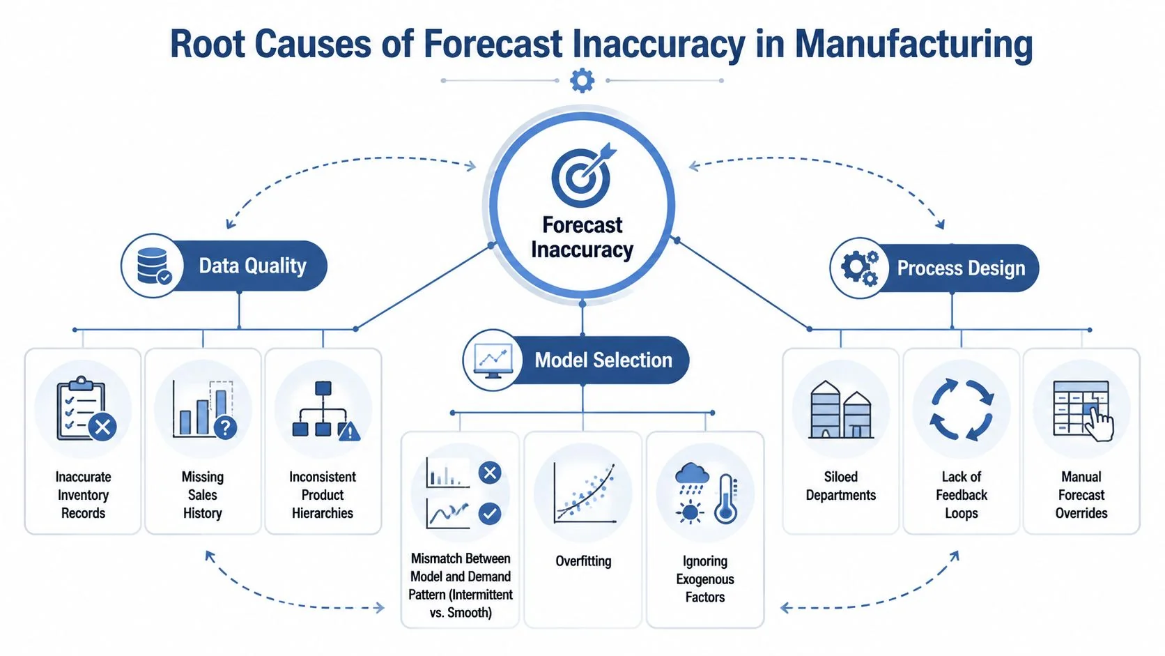
Forecast inaccuracy usually emerges from the interaction of data quality, model selection, and process design. Treating these as separate technical problems leads to partial fixes. A clean dataset won't rescue a model that misunderstands intermittent demand, and a strong model won't compensate for sales history distorted by stockouts.
Data quality comes first
The demand history may record shipments rather than unconstrained demand. When a component was unavailable, recorded sales can fall even though customer need remained high. Missing stockout flags, substitutions, returns, late postings, and inconsistent units can contaminate training data before model selection begins.
Diagnostic signals include sudden demand drops during known shortages, unexplained shifts after ERP changes, and different totals between sales, inventory, and production systems. Check product hierarchies as well. A changing SKU-to-family mapping can make a stable business look like a changing demand pattern.
Match the model to the demand
A 2025 study found that no single model performs best across all SKUs. Machine learning with exogenous features worked better for stable, high-volume items, while simpler statistical models or domain heuristics performed better for low-volume or erratic demand (context-dependent forecasting research).
That finding supports a portfolio architecture rather than a universal algorithm. Use demand classification to identify intermittent, lumpy, seasonal, trending, and stable items, then validate model families within each class. Watch for overfitting when a model performs well in backtesting but fails after promotions, assortment changes, or supplier constraints shift the data.
Process design determines whether improvements persist
Sales, marketing, procurement, and operations may work from different horizons and assumptions. A sales team may include an expected customer win that production hasn't validated, while a planner may override a statistical forecast based on a recent order that won't repeat.
Useful diagnostic signals include repeated manual overrides in one direction, large differences between statistical and consensus forecasts, and forecast changes that aren't recorded with a reason. Establish a formal override policy, capture the adjustment, and compare the edited forecast with the untouched baseline after demand is realized.
Operational test: If a forecast improvement can't be traced to better purchasing, scheduling, inventory, or service decisions, the team has improved a report rather than the planning system.
Practical Strategies to Improve Forecast Accuracy
Improvement should follow demand type. A stable, high-volume finished good and an intermittent maintenance part don't deserve the same model, data budget, or accuracy threshold.
| Demand Type | Recommended Strategy | Expected MAPE Improvement | Implementation Complexity | Key Prerequisite |
|---|---|---|---|---|
| Stable, high-volume | Exponential smoothing ensembles, hierarchy-aware reconciliation, and external feature testing | Measure against the current baseline rather than assuming a fixed lift | Moderate | Reliable history and consistent hierarchy |
| Seasonal or promotional | Model event calendars, price changes, and promotion timing explicitly | Validate by event class and forecast horizon | Moderate to high | Complete promotion and pricing records |
| Intermittent spare parts | Croston-style methods, occurrence-versus-size modeling, and service-policy tuning | Evaluate with metrics that don't punish zero-demand periods unfairly | Moderate | Correct stockout and demand-occurrence data |
| Lumpy, low-volume components | Domain heuristics, pooled related-item signals, and conservative inventory policies | Compare against a simple baseline and operational outcomes | Moderate | Product relationships and planner review |
| New products | Analog-item models, structured judgment, and scenario ranges | Establish a launch baseline instead of forcing mature-item targets | High | Credible analogs and launch assumptions |
The table intentionally avoids promising a fixed improvement percentage. There is no universal gain because performance depends on demand volatility, data richness, horizon, and the quality of the incumbent process. A team should calculate the improvement against a naive or existing production baseline, then test whether the gain survives execution constraints.
Where statistical methods work
For high-volume stable items, exponential smoothing and model ensembles are often strong starting points because they capture level, trend, and seasonality without unnecessary complexity. Hierarchical reconciliation can help keep plant, product-family, and SKU forecasts coherent, but validate whether the reconciled output improves the level where production decisions happen.
For intermittent demand, separate two questions: will demand occur, and how much will it be if it occurs? Croston variants address intermittent patterns directly, while a classifier-plus-regressor design can use different signals for occurrence and magnitude. Neither approach should be selected from leaderboard performance alone. Compare service outcomes, inventory exposure, and planner usability.
Use features only when they earn their maintenance cost
Point-of-sale data can improve visibility into downstream consumption, while weather, macroeconomic indicators, and production schedule changes may explain demand shifts in relevant industries. Add a feature only when its data is timely, stable, governed, and available at forecast creation time. Leakage from future information can make validation look impressive while offering no live value.
Human judgment remains useful for launches, supply disruptions, and one-off customer events. Use forecast value added to identify which planners, item classes, or event types benefit from intervention. The result may justify fewer overrides, not more.
For inventory decisions, connect the forecasting layer to AI inventory management practices, where forecast uncertainty can inform buffers and replenishment rather than being treated as a standalone score.
Measuring and Monitoring Accuracy Over Time
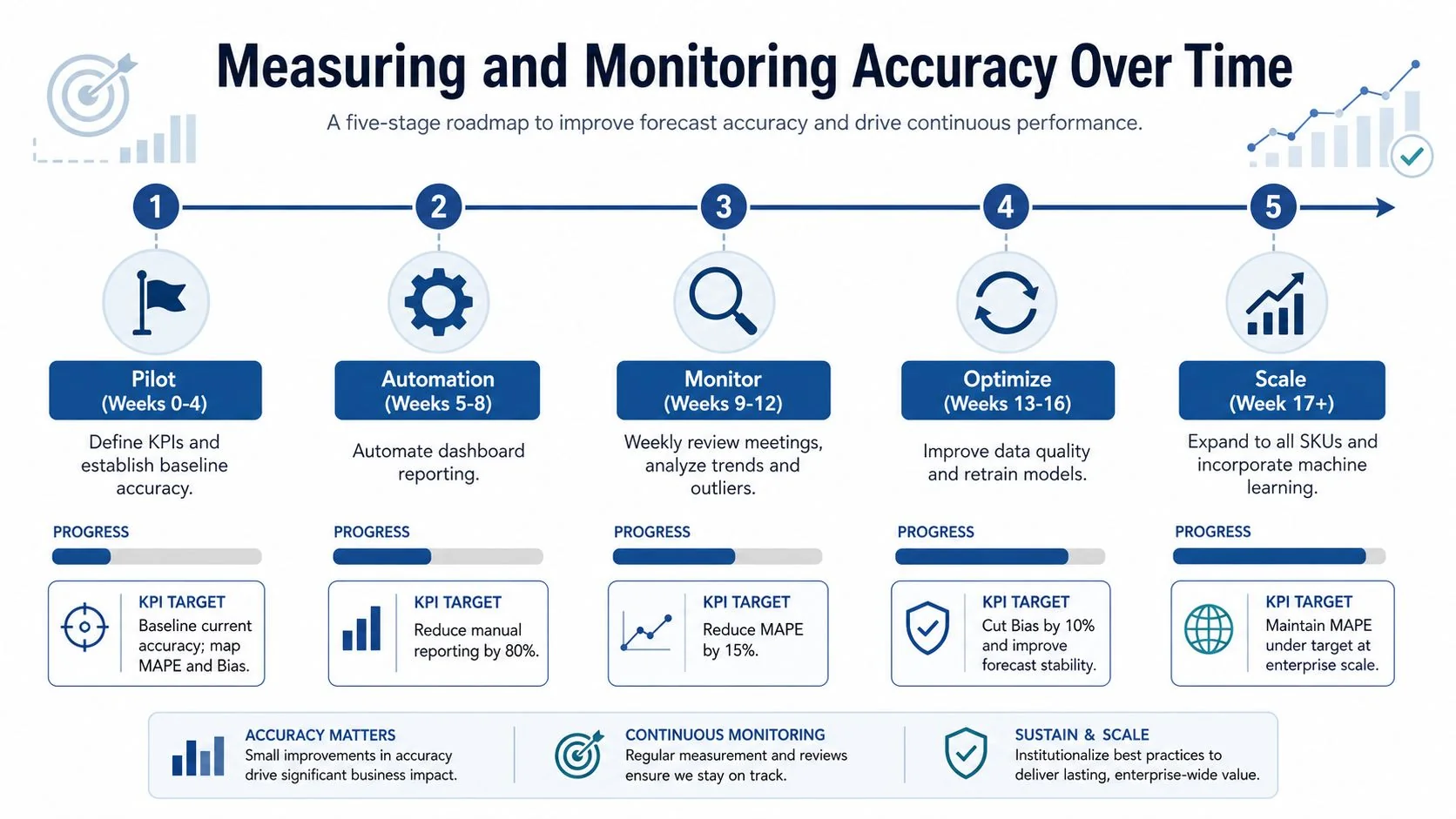
A production forecasting model needs a monitoring service, not a quarterly spreadsheet. Start with a bounded pilot, preserve the forecast version that existed when the decision was made, and compare it with realized demand at the same SKU-location-horizon level.
A pilot-to-scale operating rhythm
- Pilot: Select representative items and establish baseline MAPE, WAPE, MAD, RMSE, and bias. Include a naive benchmark.
- Validate: Separate stable, seasonal, intermittent, and new items. Confirm that improvements hold across time windows and aren't caused by aggregation.
- Integrate: Send outputs into planning workflows and measure order changes, schedule stability, inventory movement, and service outcomes.
- Operate: Automate scorecards, exception alerts, model drift checks, and retraining decisions.
- Scale: Expand only after data lineage, ownership, override logging, and downstream consumption are reliable.
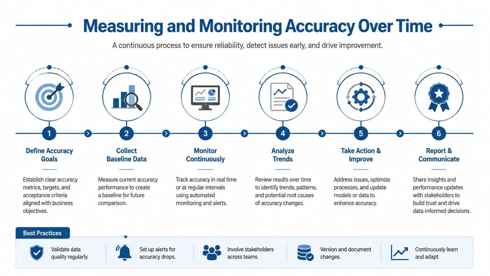
The dashboard should show rolling error, WAPE, bias, forecast value added, stockout frequency, fill rate, excess inventory, and order variability. Set thresholds by segment rather than forcing one enterprise target. Stable high-volume products can reasonably target the higher end of the 75% to 85% accuracy range, while slow-moving items require more tolerant expectations (forecast measurement guidance).
Assign one owner for the accuracy scorecard and separate responsibilities for data quality, model performance, and planning adoption. A drift alert should trigger investigation, not automatic retraining in every case. Retrain when the data pipeline is sound and the demand pattern has changed. Escalate to model redevelopment when errors persist after data and process corrections.
A supply chain control tower approach can provide the cross-functional visibility needed to connect forecast exceptions with supplier, inventory, production, and service signals.
Connecting Forecast Accuracy to Manufacturing AI Success
Demand forecasting accuracy is a prerequisite capability for manufacturing AI because production scheduling, inventory optimization, procurement automation, and capacity planning all depend on a reliable demand signal. A model that predicts demand well but isn't consumed by MRP, safety-stock policy, or planner workflows won't create plant value.
The practical sequence is clear: clean the demand history, segment items by behavior, choose metrics that match decisions, control human overrides, and monitor downstream execution. Use AI where the data contains repeatable signal and the process can act on uncertainty. Use simpler models or structured human judgment where demand is sparse, new, or dominated by one-off events.
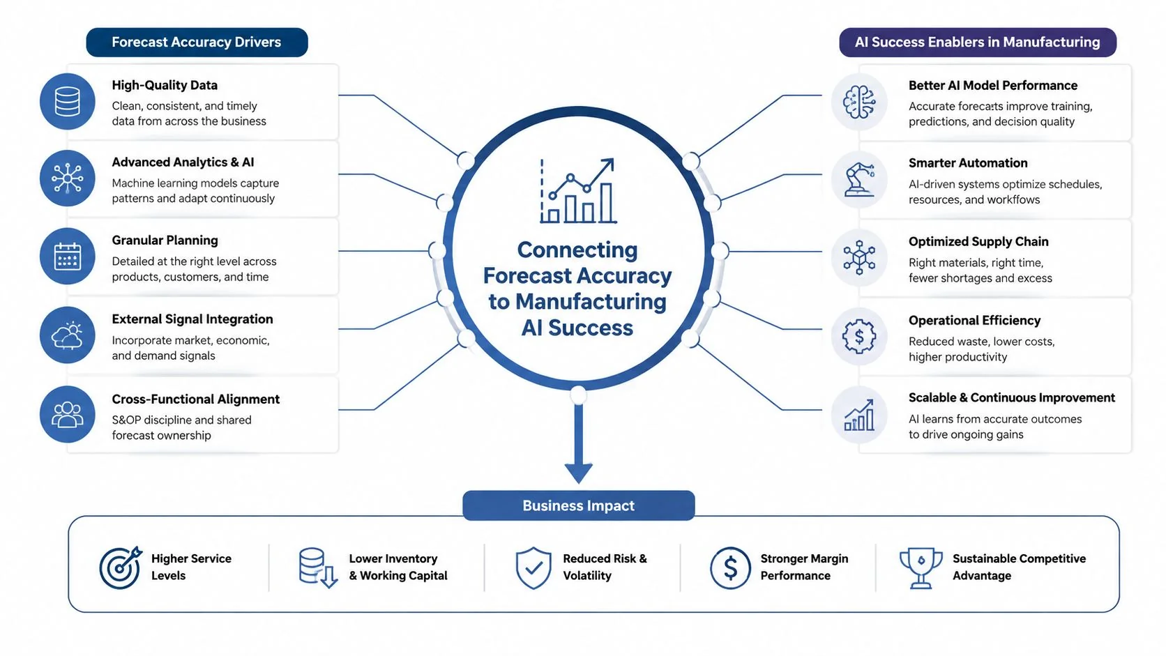
Start your next manufacturing AI initiative by auditing forecast versions, stockout data, overrides, and SKU-location metrics. Then pilot one demand segment, connect its forecast to a real planning decision, and measure both statistical error and execution stability before expanding.
If your team is evaluating demand forecasting, inventory, or other factory AI use cases, review documented implementations in the AI for Manufacturing case-study database, compare evidence levels and operational outcomes, and use those findings to define a pilot with measurable decision-level KPIs.
