Define Process Optimization for Manufacturing AI Use
Define process optimization for manufacturing AI with objectives, Lean and Six Sigma methods, KPIs, pitfalls, an AI evaluation checklist, and real case
Written by AI for Manufacturing
Process optimization in manufacturing is the systematic adjustment of process variables to maximize throughput, quality, yield, or resource efficiency within defined constraints. It means improving a repeatable operating point, not pushing a machine to run faster.
Factories can lose 20% to 30% of productive capacity through inefficiencies, rework, and downtime, and optimization efforts still fail when they chase local speed instead of total plant performance, as reported in the manufacturing optimization overview from Advanced Technology Services. For manufacturing AI, the practical scope is clear: define the loss, identify the controllable lever, set hard operating limits, and measure whether the gain survives ordinary production variation.
Table of Contents
- What Process Optimization Actually Means in Manufacturing
- How the Discipline Evolved from Lean to AI
- Main Methods Used on the Plant Floor
- Key KPIs That Make Optimization Measurable
- When to Optimize and Where to Stop
- Evaluating AI-Enabled Optimization Solutions
- Manufacturing Case Examples With Measured Outcomes
- Connecting Process Optimization to AI in Manufacturing
What Process Optimization Actually Means in Manufacturing
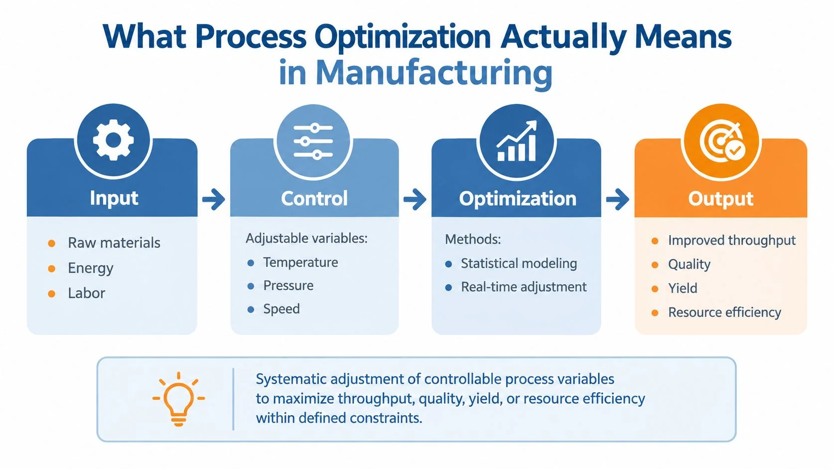
To define process optimization accurately, start with the process variables operators and engineers can change. These may include temperature, pressure, line speed, feed rate, recipe settings, maintenance timing, staffing, sequencing, or production scheduling. The optimization target might be throughput, yield, quality, energy efficiency, or resource utilization, but every target sits inside constraints for safety, product specifications, capacity, cost, delivery, and workforce conditions.
That makes optimization a constrained quantitative discipline, not a general productivity slogan. A line that produces more units but creates unacceptable scrap hasn't been optimized. A machine that consumes less energy but causes longer recovery periods may only have shifted the loss. The useful definition of process optimization therefore includes both the desired output and the boundaries that cannot be violated.
A practical optimization cycle
A sound project normally follows a repeatable sequence:
- Establish the baseline. Record current performance using consistent definitions for downtime, scrap, rework, cycle time, and good output.
- Find the dominant loss. Separate the main constraint from secondary symptoms. A bottleneck, quality excursion, or changeover issue deserves a different intervention.
- Test a controlled change. Adjust a defined variable under a known operating envelope instead of changing several conditions at once.
- Verify and standardize. Confirm the result across normal product and shift variation, then update standard work, controls, training, and monitoring.
A useful optimization project has a named owner, finite scope, and explicit trade-offs. The practical output might be a revised recipe, setpoint, schedule, workflow, or control policy, supported by evidence that it works beyond a single favorable run. Teams beginning an AI initiative can use the process optimization benchmarks as a reference point for structuring measurable objectives, but the plant's own baseline remains the governing evidence.
Practical rule: If you can't name the controllable variable and the constraint it must respect, you haven't defined an AI optimization problem yet.
How the Discipline Evolved from Lean to AI
Manufacturing optimization developed by making previously invisible losses easier to see and control. In the postwar Japanese industrial system, Lean manufacturing gave factories a practical way to improve flow by reducing waste, queues, unnecessary movement, setup delays, and work that didn't add customer value. This history is documented in the manufacturing process optimization overview from 4U Machining.
Six Sigma added a stronger statistical lens. Motorola introduced Six Sigma in 1986, and the approach became widely popular across global industry during the 1990s, according to the same historical account. Lean concentrates on flow and waste, while Six Sigma concentrates on variation and defects. The commonly cited Six Sigma benchmark is 3.4 defects per million opportunities, a target also described by the American Society for Quality.
Each method expanded what plants could measure
The progression matters for AI deployment because each stage solves a different visibility problem:
- Lean and standard work show where people, materials, and machines wait or move unnecessarily.
- Statistical process control and Six Sigma connect process inputs with variation and defects.
- Manufacturing execution and historian systems create detailed records of machine states, recipes, quality results, and production events.
- Process mining reconstructs the route work followed, including queues, rework loops, and deviations from intended sequencing.
- AI and machine learning estimate complex relationships across sensor, quality, maintenance, and scheduling data.
AI doesn't replace the earlier disciplines. Lean helps define waste, Six Sigma helps verify causes and capability, process mining reveals actual behavior, and machine learning can support prediction, recommendation, optimization, or closed-loop control. Without stable definitions and trustworthy event data, an advanced model often learns historical workarounds rather than the process engineers intend to operate.
For teams building an AI roadmap, manufacturing data analytics is most useful when it supports a specific decision, such as changing a setpoint or prioritizing maintenance, rather than becoming a dashboard exercise.
Main Methods Used on the Plant Floor
Lean, Six Sigma, process mining, and AI/ML shouldn't be treated as interchangeable labels. Each method fits a different type of loss and fails in a different way.
| Method | Best at optimizing | Typical plant-floor evidence | Common limitation |
|---|---|---|---|
| Lean | Flow, setup, waiting, motion, standard work, and visible waste | Value-stream maps, time observations, kanban signals, changeover records | May remove obvious waste without proving the cause of complex variation |
| Six Sigma | Defects, variation, capability, and repeatability | Control charts, measurement-system studies, quality records, designed tests | Can be slow and data-intensive when measurement or sponsorship is weak |
| Process mining | Actual routes, queues, rework loops, and bottlenecks | MES, quality, maintenance, and event timestamps | Shows what happened, but not necessarily why it happened |
| AI/ML | Prediction, anomaly detection, classification, recommendations, and multivariable control | Sensor histories, PLC tags, recipes, schedules, inspection results | Requires representative data, constraints, drift monitoring, and safe fallbacks |
Lean tools such as value-stream mapping, 5S, SMED, kanban, standard work, and mistake-proofing work well when the problem is visible and procedural. A changeover reduction project rarely needs a neural network before engineers have observed the work and removed unnecessary steps.
Six Sigma is stronger when a quality or yield problem has multiple interacting inputs. Measurement-system analysis matters because a model can't compensate for unreliable labels or inconsistent inspection. Control charts and statistical testing also help distinguish common process noise from assignable causes.
Process mining is valuable when teams disagree about how work really flows. It can expose rework paths or queue accumulation hidden by average cycle-time reporting, but engineers still need process knowledge to test the cause.
AI earns its place when the decision spans too many variables for manual rules. It may recommend a recipe, schedule, inspection policy, or maintenance action, but it must connect to a real actuator or operating decision. Combining methods is usually stronger than selecting one fashionable tool.
Key KPIs That Make Optimization Measurable
Overall Equipment Effectiveness, or OEE, gives optimization a practical baseline by separating performance into Availability × Performance × Quality, as shown in this guide to calculating OEE. Availability covers downtime and changeovers, Performance captures speed losses and micro-stoppages, and Quality includes scrap and rework. The breakdown connects each loss to a controllable lever and helps determine whether AI should predict downtime, detect speed instability, or improve inspection decisions.
A commonly cited world-class OEE benchmark is 85%, according to Intelycx's explanation of process optimization in manufacturing. It is not a universal production requirement. The value lies in the decomposition. Raising one component while another deteriorates can hide a shifted loss, so teams should review OEE alongside output, quality, and resource use.
Match each KPI to a lever
Use a focused KPI set that matches the decision under optimization:
- First Pass Yield: Directs recipe, parameter, and inspection changes toward units accepted without rework.
- Throughput: Tests whether a change raises total good output instead of only local machine speed.
- Cycle-time variation: Exposes instability that averages conceal and provides a useful AI prediction target.
- Mean Time Between Failures: Links reliability actions to operating conditions and maintenance timing.
- Scrap cost per unit: Converts quality loss into an economic priority.
- Energy per good unit: Checks whether higher output requires excessive resource consumption.
Each KPI needs consistent event and quality definitions. If shifts classify downtime differently, an AI model may optimize reporting behavior rather than equipment performance. Use the same loss categories in training, validation, and post-deployment monitoring. This consistency also determines whether a recommendation can be trusted by operators and engineers.
A documented production example reported more than €60,000 per year in electricity savings after peak-load optimization tied to OEE tracking, as described by Intelycx. That result should not become a promise for every line. It demonstrates the better evaluation method: connect energy decisions to good output and an established production KPI, then judge the AI intervention against both.
When to Optimize and Where to Stop
More optimization isn't automatically better. Start only after the baseline is stable enough to distinguish a real improvement from measurement noise, and after the bottleneck is identified in terms the plant can observe.
Three failure modes deserve attention
Local optimization occurs when one machine runs faster but the next process can't consume its output. The upstream OEE may improve while downstream starvation, blocking, work-in-process, or total delivery performance worsens.
Shifted bottlenecks appear when a team removes one constraint and moves the limiting condition to a less instrumented station. The plant may report a better local KPI while visibility drops exactly where the next loss begins.
Operator burden grows when recommendations arrive faster than people can verify and apply them. Operators then create workarounds, ignore alerts, or lose confidence in a system that doesn't respect the practical rhythm of the line.
AI amplifies these traps because it can iterate faster than legacy review cycles.
Use a stopping rule before deployment. Freeze a change when marginal gain per engineering hour falls below the cost of monitoring drift, or when the change degrades safety, the quality floor, ergonomics, or reliable delivery. A recommendation that improves a narrow objective but increases review effort isn't a durable optimization.
The system boundary also matters. Include machines, quality control, maintenance, labor, scheduling, and downstream capacity when evaluating an intervention. Local gains are acceptable only when the plant can show that they improve the constrained outcome the customer and operations team care about.
Evaluating AI-Enabled Optimization Solutions
Vendor evaluation should focus on whether the system can make a safe, auditable decision from plant data. A polished demo doesn't establish that the model will work after recipes, products, sensors, and operating conditions change.
Data and ground truth
Ask whether the historical record contains process parameters and verified outcomes, or only recent logs and operator comments. Require time-based train and test separation so the evaluation resembles deployment, then define how the team will detect drift in sensors, recipes, products, and production mix.
Mechanism and constraints
The solution should identify the controllable levers behind its recommendation. Safety limits, quality floors, capacity restrictions, and throughput requirements should act as hard constraints where appropriate, not merely soft penalties inside an opaque score.
Durability and operability
Test missing sensors, changed recipes, new products, delayed laboratory results, and degraded connectivity. Plant engineers should be able to review every proposed setpoint before it reaches the line, with a clear fallback to a known safe operating policy.
Commercial and integration claims
Request a paid pilot on a non-hero asset, define KPIs before the pilot begins, and include a holdout period after training. Require a written remediation plan for model failure, not just a promise of support.
Reject demonstrations based solely on synthetic data or a single favorable shift. Tools such as the AI for Manufacturing case-study database can help teams compare documented use cases, technologies, industries, and reported outcomes, but procurement still needs plant-specific validation.
Manufacturing Case Examples With Measured Outcomes
The following examples illustrate how a lever, method, and KPI fit together. They aren't generic promises for every factory. Each result depends on the process, data quality, implementation discipline, and operating constraints involved.
| Case | Method | Lever | KPI Movement | Measured Result |
|---|---|---|---|---|
| Discrete assembly cell | Standard work, cycle-time analytics, and AI classification | Micro-stop identification from PLC tags | OEE | Increased from 58% to 71% in 14 weeks |
| Semiconductor fabrication tool | Process mining and multivariate SPC | Lithography process monitoring | Excursion rate and wafer yield | Excursion rate reduced 42%, wafer yield reclaimed 6.2% |
| Batch chemical line | Hybrid mechanistic and ML model | Operating conditions affecting energy demand | Energy per ton | Reduced 11% without violating quality specifications |
In the assembly cell, conventional engineering did much of the foundational work. Standard work established a consistent operating method, and cycle-time analysis exposed where time disappeared. AI helped classify micro-stops from PLC tags, turning ambiguous short interruptions into categories the team could act on. The measured OEE movement was from 58% to 71% in 14 weeks, as reported for this deployment.
The semiconductor example used process mining to reconstruct tool behavior and multivariate statistical process control to connect operating conditions with excursions. The combined method mattered because it linked event sequences and interacting variables to a specific quality and yield decision.
The chemical example used a hybrid model rather than relying on machine learning alone. Mechanistic knowledge supplied process boundaries, while ML represented relationships difficult to encode manually. Energy per ton fell 11% without violating quality specifications, showing why a resource objective needs explicit product constraints.
Across the three cases, AI moved the needle where the decision was multivariable, repetitive, and measurable. Conventional engineering remained responsible for defining the process, limits, standard work, and acceptance criteria.
Connecting Process Optimization to AI in Manufacturing
To define process optimization for an AI project, write down four things before selecting a model: the loss category, the controllable lever, the hard constraints, and the KPI that proves the change worked.
A practical next-week sequence is:
- Audit the current loss categories using the OEE decomposition of availability, performance, and quality.
- Match each loss to the right method. Use Lean for visible flow waste, Six Sigma for variation, process mining for unclear event paths, and AI for complex repeatable decisions.
- Score candidate solutions against data quality, constraint handling, drift response, auditability, integration, and failure recovery.
- Instrument the chosen KPI so the model is trained and evaluated against the same loss bucket plant leaders already use.
AI earns its place only after the quantitative framing is settled. Without a defined operating boundary, a model may optimize speed at the expense of quality, energy, safety, or downstream capacity, and operators will correctly reject it.
Start with one constrained decision on one measurable loss. Document the baseline, run a controlled pilot, review the result with operators and engineers, and expand only when the gain remains durable under normal production conditions.
If you're evaluating an AI manufacturing initiative now, map your line's largest OEE loss to a controllable variable, define its quality and safety limits, and use that specification to compare vendors or documented implementations before approving a pilot.
